SVMs - Part II (Application)
Now that we have the theory of Support Vector Machines, I am now going to code a Support Vector Machine from Scratch. First, I am going to start with some data.
import cvxpy as cp
import pandas as pd
import matplotlib.pyplot as plt
from sklearn.datasets import make_blobs
import numpy as np
# create dataset
data, labels = make_blobs(n_features=2, centers=2, cluster_std=1.25,
                          random_state=11, n_samples = 10)
df = pd.DataFrame({'Credit Score': data[:, 0], 'Income': data[:, 1],
                   'Target': labels})

with plt.style.context('fivethirtyeight'):
    fig, ax = plt.subplots(figsize = (8, 8))
    df[df['Target'] == 0].plot(x = 'Credit Score', y = 'Income', color = 'red',
                              kind = 'scatter', ax = ax,
                              s = 100, label = 'default')
    df[df['Target'] == 1].plot(x = 'Credit Score', y = 'Income', color = 'blue',
                              kind = 'scatter', ax = ax,
                              s = 100, label = 'repaid')
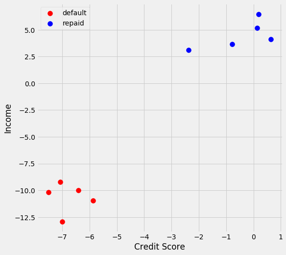
I am going to predict whether someone repays or defaults on their loan based on their credit score and income. In this instance, the data has been scaled. We see with this problem I can use a hard classifier because there is a clear seperation between the 2 classes.
I am going to convert the target variable to be 1 and -1 so that I can utilize this formula:
\((a_1x_{1j} + a_2x_{2j} + ... + a_mx_{mj} + a_0)y_j \geq 1\)
df['Target'] = df['Target'].map(lambda x: -1 if x == 0 else x)
df
| Credit Score | Income | Target | |
|---|---|---|---|
| 0 | -0.774473 | 3.644370 | 1 |
| 1 | -7.502406 | -10.205162 | -1 |
| 2 | 0.633908 | 4.111708 | 1 |
| 3 | -7.000313 | -12.927143 | -1 |
| 4 | -6.404962 | -10.010034 | -1 |
| 5 | -2.367565 | 3.099335 | 1 |
| 6 | -5.868293 | -10.942499 | -1 |
| 7 | -7.065393 | -9.216242 | -1 |
| 8 | 0.185417 | 6.466971 | 1 |
| 9 | 0.126473 | 5.200169 | 1 |
Solving for a support vector machine is a classic optimization problem. An optimization problem consists of 3 parts - variables, constraints, and objective function. For this specific problem they are as follows:
- Variables: I am looking for values for each of the coefficients (Credit Score and Income) and a value for the intercept (\(a_1\), \(a_2\), and \(a_0\))
- Constraints: Since I am going to be using a hard classifier I need to find values for each coefficient that allows for each point to be on the correct side of the classifier (\((a_1x_{1j} + a_2x_{2j} + ... + a_mx_{mj} + a_0)y_j \geq 1\))
- Objective Function: I want to maximize the margin of the classifier. To do this I need to minimize \(\sum_i(a_i)^2\)
I am now going to code this out using the CVXPY library used for solving convex optimization problems.
# Make variables
a0 = cp.Variable()
a1 = cp.Variable()
a2 = cp.Variable()
# Make constraints
constraints = []
for index, row in df.iterrows():
    constraints.append(((row['Credit Score'] * a1) + \
                (row['Income']) * a2 + a0) * row['Target'] >= 1)
# Make objective function
obj = cp.Minimize((a1**2) + (a2**2))
svm_prob = cp.Problem(obj, constraints)
svm_prob.solve()
svm_prob.status
'optimal'
This means that our optimizer successfully found variables (\(a_1, a_2, a_0)\) that met all of our constraints. Now I will take a look at what these variables are.
a0.value, a1.value, a2.value
(array(0.6886473), array(0.05407789), array(0.14176774))
I am now going to plot my classifier. To do this I know the equation of the line is \(Credit Score * a_1 + Income * a_2 + a_0 = 0\). To solve for income the equation becomes
\(Income = \dfrac{-Credit Score * a_1 - a_0}{a_2}\)
vals = []
for index, row in df.iterrows():
    vals.append((((-row['Credit Score'] * a1.value) - a0.value) / a2.value))
with plt.style.context('fivethirtyeight'):
    fig, ax = plt.subplots(figsize = (8, 8))
    df[df['Target'] == -1].plot(x = 'Credit Score', y = 'Income', color = 'red',
                              kind = 'scatter', ax = ax,
                              s = 100, label = 'default')
    df[df['Target'] == 1].plot(x = 'Credit Score', y = 'Income', color = 'blue',
                              kind = 'scatter', ax = ax,
                              s = 100, label = 'repaid')
    plt.plot(df['Credit Score'], vals, color = 'k', label = 'Classifier')
    plt.legend()
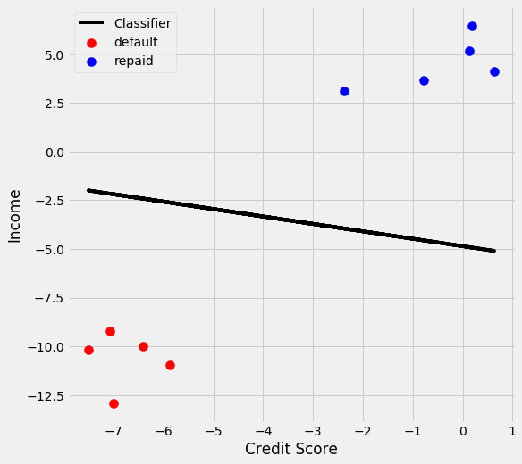
We see the classifier in relation to the two categories and see that it does a good job of classifying the two categories. Now I want to find the support vectors. The support vector for the positive class is
\(Credit Score * a_1 + Income * a_2 + a_0 = 1\)
The support vector for the negative class is
\(Credit Score * a_1 + Income * a_2 + a_0 = -1\)
vals = []
upper_support = []
lower_support = []
for index, row in df.iterrows():
    vals.append((((-row['Credit Score'] * a1.value) - a0.value ) / a2.value))
    upper_support.append((((-row['Credit Score'] * a1.value) - \
                  a0.value + 1) / a2.value))
    lower_support.append((((-row['Credit Score'] * a1.value) - \
                  a0.value - 1) / a2.value))
with plt.style.context('fivethirtyeight'):
    fig, ax = plt.subplots(figsize = (8, 8))
    df[df['Target'] == -1].plot(x = 'Credit Score', y = 'Income', color = 'red',
                              kind = 'scatter', ax = ax,
                              s = 100, label = 'default')
    df[df['Target'] == 1].plot(x = 'Credit Score', y = 'Income', color = 'blue',
                              kind = 'scatter', ax = ax,
                              s = 100, label = 'repaid')
    plt.plot(df['Credit Score'], vals, color = 'k')
    plt.plot(df['Credit Score'], upper_support, color = 'green')
    plt.plot(df['Credit Score'], lower_support, color = 'green')
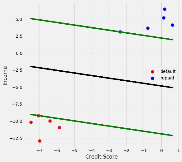
Remaking the graph with the support vectors we can see the margin between the 2 classifiers. The optimization problem successfully found the line that would maximize the margin between the 2 classes. I want to see how my model does versus the implementation of sklearn’s support vector classifier.
from sklearn.svm import SVC
svm = SVC(kernel = 'linear', C = 1E100)
I am using a linear kernel and a very large C value. This is because I used a linear classifier and I used a hard classifier, as C increases the importance of finding as many values correct outweighs the importance of finding a classifier that maximizes the margin.
svm.fit(df.drop('Target', axis = 1), df['Target'])
SVC(C=1e+100, cache_size=200, class_weight=None, coef0=0.0,
    decision_function_shape='ovr', degree=3, gamma='auto_deprecated',
    kernel='linear', max_iter=-1, probability=False, random_state=None,
    shrinking=True, tol=0.001, verbose=False)
Model has been fit. Lets see what the coefficients and intercept are
svm.coef_, svm.intercept_
(array([[0.05407789, 0.14176774]]), array([0.68864728]))
# my coefficeints and intercepts
a1.value, a2.value, a0.value
(array(0.05407789), array(0.14176774), array(0.6886473))
We see that they are almost exactly the same number!
Interpretting the Results
A big part of machine learning is making sure that you understand your model. What do the values of the coefficients mean? Credit Score has a coefficient of 0.05 and income has a coefficient of 0.14. Income’s coefficient is almost 3 times larger than credit score’s coefficient. This implies that income is a more important predictor of whether someone will repay a loan than credit score (remember this is randomly generated data). Lets explore this.
diff_credit_score = df[df['Target'] == 1]['Credit Score'].median() - \
                    df[df['Target'] != 1]['Credit Score'].median()
diff_income = df[df['Target'] == 1]['Income'].median() - \
              df[df['Target'] != 1]['Income'].median()

with plt.style.context('fivethirtyeight'):
    fig, ax = plt.subplots(figsize = (8, 8))
    ax.bar(['Credit Score', 'Income'], [diff_credit_score, diff_income])
    ax.set_title('Median Difference Between Income and Credit Score')
    ax.set_ylabel('Median Difference')
    ax.text(-.1, 6, np.round(diff_credit_score, 2), fontsize = 18)
    ax.text(.9, 13, np.round(diff_income, 2))
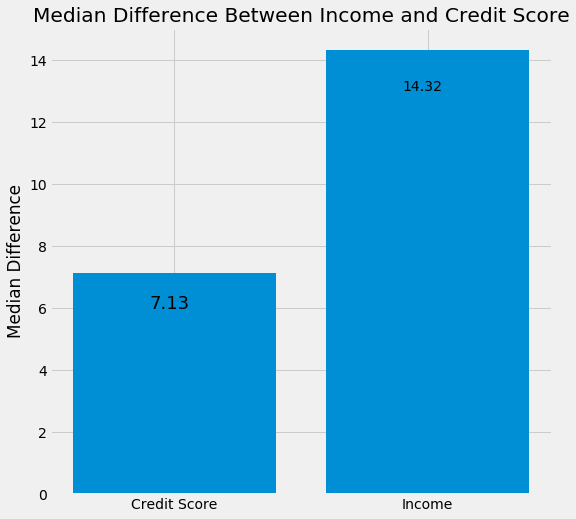
We see that the median difference between the two classes for credit score is 7 and the median difference between the two classes for income is 14. So, the difference is much larger in income and the coefficent also supports that income is a more important variable than credit score.
Now lets try out a dataset that a linear classifier would not be useful.
data, labels = make_blobs(n_features=2, centers=2, cluster_std=11,
                          random_state=11, n_samples = 10)
df = pd.DataFrame({'Credit Score': data[:, 0], 'Income': data[:, 1],
                  'Target': labels})

with plt.style.context('fivethirtyeight'):
    fig, ax = plt.subplots(figsize = (8, 8))
    df[df['Target'] == 0].plot(x = 'Credit Score', y = 'Income', color = 'red',
                              kind = 'scatter', ax = ax,
                              s = 100, label = 'default')
    df[df['Target'] == 1].plot(x = 'Credit Score', y = 'Income', color = 'blue',
                              kind = 'scatter', ax = ax,
                              s = 100, label = 'repaid')
# Make sure target variable is 1 and -1
df['Target'] = df['Target'].map(lambda x: -1 if x == 0 else x)
df
| Credit Score | Income | Target | |
|---|---|---|---|
| 0 | -1.077455 | -3.019234 | 1 |
| 1 | -16.143243 | -14.843564 | -1 |
| 2 | 11.316297 | 1.093336 | 1 |
| 3 | -11.724823 | -38.796999 | -1 |
| 4 | -6.485737 | -13.126440 | -1 |
| 5 | -15.096663 | -7.815549 | 1 |
| 6 | -1.763048 | -21.332128 | -1 |
| 7 | -12.297529 | -6.141066 | -1 |
| 8 | 7.369582 | 21.819653 | 1 |
| 9 | 6.850876 | 10.671793 | 1 |
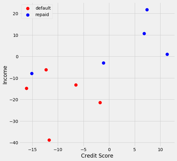
We see that we will not be able to fit a straight line through this dataset and have all the points will be on the correct side of the line. We will not be able to find a line that would meet our constraint of \((a_1x_{1j} + a_2x_{2j} + ... + a_mx_{mj} + a_0)y_j \geq 1\) With that being said, let’s see what happens if we try.
# Make variables
a0 = cp.Variable()
a1 = cp.Variable()
a2 = cp.Variable()
# Make constraints
constraints = []
for index, row in df.iterrows():
    constraints.append(((row['Credit Score'] * a1) + \
    (row['Income']) * a2 + a0) * row['Target'] >= 1)
# Make objective function
obj = cp.Minimize((a1**2) + (a2**2))
svm_prob_2 = cp.Problem(obj, constraints)
svm_prob_2.solve()
svm_prob_2.status
'infeasible'
We see that the results of this is infeasible, which is to be expected. Now I am going to try a soft classifer, where I am all right with a few misclassifications assuming I can maximize the margin.
Soft Classifier
For a soft classifier we will need to change our variables, constraints, and objective function of the classifier. Let’s start with the constraint: \((a_1x_{1j} + a_2x_{2j} + ... + a_mx_{mj} + a_0)y_j \geq 1 - \xi\)
This formula has a new variable \(\xi\). If the point is on the correct side of the line then, \(\xi\) will be 0, however if it is on the wrong side of the line then there will be a value for \(\xi\) so that the constraint is still accurate. The larger the value for \(\xi\) the larger the error. This then leads to the objective function: Minimize \(\sum_i(a_i)^2 + C(\sum_i \xi^{(i)})\) C is a value to specify to trade off between maximizing the margin and minimizing mistakes. A low value for C means that our classifier is prioritizing a large margin and a large value for C means that our classifier is prioritizing minimizing the number of mistakes.
I’m now going to walk through all 3 parts of my optimization function starting with the variables. I will need the following variables:
- \(a_1\): coefficient for credit score
- \(a_2\): coefficient for income
- \(a_0\): intercept
- \(\xi\): amount each point is off (note there will be a \(\xi\) for each data point).
Coding this will be as follows:
# variables
a0 = cp.Variable()
a1 = cp.Variable()
a2 = cp.Variable()
ksi = cp.Variable(10)
I have the following constraints:
\((a_1x_{1j} + a_2x_{2j} + ... + a_mx_{mj} + a_0)y_j \geq 1 - \xi\)
\(\xi \geq 0\)
I need \(\xi\) to be greater than or equal to be zero. I have to specify this or the optimizer will “cheat” and make some of the \(\xi\) variable negative. Coding this will be as follows:
# the constraints
constraints_coef = []
for index, row in df.iterrows():
    constraints_coef.append(((row['Credit Score'] * a1) + \
                             (row['Income']) * a2 + a0) * row['Target'] >= 1 \
                                                                - ksi[index])
ksi_constraints = [ksi >= 0 for x_i in range(100)]

constraints = constraints_coef + ksi_constraints
Finally, like I mentioned earlier my objective function is:
Minimize \(\sum_i(a_i)^2 + C(\sum_i \xi^{(i)})\) To code that is as follows (going to specify C = 1):
C = 1
soft_objective = cp.Minimize(((a1**2) + (a2**2)) + C*(sum(ksi)))
soft_classifier = cp.Problem(soft_objective, constraints)
soft_classifier.solve(solver = 'ECOS')
soft_classifier.status
'optimal'
I now get an optimal result. Lets see how the graph looks.
vals = []
upper_support = []
lower_support = []
for index, row in df.iterrows():
    vals.append((((-row['Credit Score'] * a1.value) - a0.value) / a2.value))
    upper_support.append((((-row['Credit Score'] * a1.value) - \
                            a0.value + 1) / a2.value))
    lower_support.append((((-row['Credit Score'] * a1.value) - \
                            a0.value - 1) / a2.value))

with plt.style.context('fivethirtyeight'):
    fig, ax = plt.subplots(figsize = (8, 8))
    df[df['Target'] == -1].plot(x = 'Credit Score', y = 'Income', color = 'red',
                              kind = 'scatter', ax = ax,
                              s = 100, label = 'default')
    df[df['Target'] == 1].plot(x = 'Credit Score', y = 'Income', color = 'blue',
                              kind = 'scatter', ax = ax,
                              s = 100, label = 'repaid')
    plt.plot(df['Credit Score'], vals, color = 'k')
    plt.plot(df['Credit Score'], upper_support, color = 'green')
    plt.plot(df['Credit Score'], lower_support, color = 'green')
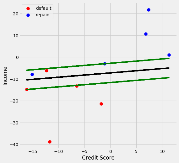
We now see that we predict one to repay their loan that acutally defaulted on their loan. I am going to turn this into a function, so that we can try out different values of C and see how the plot changes.
data, labels = make_blobs(n_features=2, centers=2, cluster_std=11,
                         random_state=11, n_samples = 10)
df = pd.DataFrame({'Credit Score': data[:, 0], 'Income': data[:, 1],
                          'Target': labels})
def soft_margin_svm(C):
    '''
    Function to solve for a soft margin support vector machine classifier

    Args
        C (float): Tradeoff between maximizing margin and minimizing mistakes.
                   Small value of C will maximize the margin and a large
                   value of C will minimize the mistakes

    Returns
        optimization model and plot showing classifier and support vectors
    '''
    data, labels = make_blobs(n_features=2, centers=2, cluster_std=11,
                              random_state=11, n_samples = 10)
    df = pd.DataFrame({'Credit Score': data[:, 0], 'Income': data[:, 1],
                       'Target': labels})
    df['Target'] = df['Target'].map(lambda x: -1 if x == 0 else x)

    # variables
    a0 = cp.Variable()
    a1 = cp.Variable()
    a2 = cp.Variable()
    ksi = cp.Variable(10)

    # the constraints
    constraints_coef = []
    for index, row in df.iterrows():
        constraints_coef.append(((row['Credit Score'] * a1) + \
                                 (row['Income']) * a2 + a0) * \
                                 row['Target'] >= 1 - ksi[index])
    ksi_constraints = [ksi >= 0 for x_i in range(100)]

    constraints = constraints_coef + ksi_constraints

    # objective function
    soft_objective = cp.Minimize(((a1**2) + (a2**2)) + C*(sum(ksi)))

    soft_classifier = cp.Problem(soft_objective, constraints)
    soft_classifier.solve(solver = 'ECOS')

    # make plot
    data, labels = make_blobs(n_features=2, centers=2, cluster_std=11,
                               random_state=11, n_samples = 10)
    df = pd.DataFrame({'Credit Score': data[:, 0], 'Income': data[:, 1],
                      'Target': labels})
    vals = []
    upper_support = []
    lower_support = []
    for index, row in df.iterrows():
        vals.append((((-row['Credit Score'] * a1.value) - a0.value) / a2.value))
        upper_support.append((((-row['Credit Score'] * a1.value) - \
                                a0.value + 1) / a2.value))
        lower_support.append((((-row['Credit Score'] * a1.value) - \
                                a0.value - 1) / a2.value))

    with plt.style.context('fivethirtyeight'):
        fig, ax = plt.subplots(figsize = (8, 8))
        df[df['Target'] == 0].plot(x = 'Credit Score', y = 'Income',
                                  color = 'red',
                                  kind = 'scatter', ax = ax,
                                  s = 100, label = 'default')
        df[df['Target'] == 1].plot(x = 'Credit Score', y = 'Income',
                                  color = 'blue',
                                  kind = 'scatter', ax = ax,
                                  s = 100, label = 'repaid')
        plt.plot(df['Credit Score'], vals, color = 'k')
        plt.plot(df['Credit Score'], upper_support, color = 'green')
        plt.plot(df['Credit Score'], lower_support, color = 'green')
        plt.title(f'C = {C}')

    return soft_classifier
soft_margin_svm(.001);
soft_margin_svm(1);
soft_margin_svm(1000);
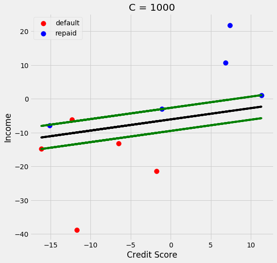
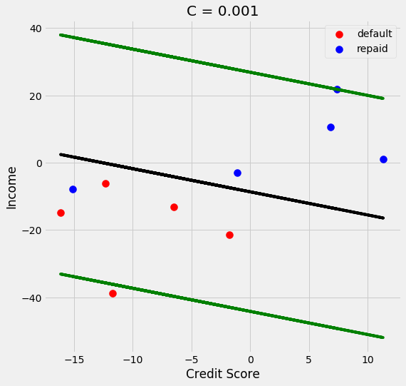
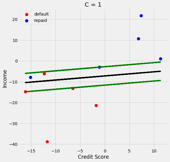
We see that as C gets larger the margin gets smaller. One more thing I want to cover is what if predicting one class is more important than predicting the other class. For example, lets say that I am very conservative and only want to give loans to people that I am very confident will repay their loans. I can change the equation of the line so that I move it away from the default class and towards the class I want to be conservative towards. To do this I change the equation of the line to be the following:
\(a_1 * credit score + a_2 * income + [\dfrac{2}{3}(a_0 + 1) + \dfrac{1}{3}(a_0 - 1)] = 0\) Which becomes: \(a_1 * credit score + a_2 * income + [a_0 + \dfrac{1}{3}] = 0\)
This implies that predicting class 1 (predicting they repaid and they don’t) is twice as costly as predicting class 1 (predicting they don’t repay and they do repay). In essence, giving a bad loan is twice as costly as withholding a good loan. Let’s see how this changes our line.
vals = []
upper_support = []
lower_support = []
classifier_unequal = []
upper_unequal = []
lower_unequal = []
for index, row in df.iterrows():
    vals.append((((-row['Credit Score'] * a1.value) - a0.value) / a2.value))
    upper_support.append((((-row['Credit Score'] * a1.value) - \
                          a0.value + 1) / a2.value))
    lower_support.append((((-row['Credit Score'] * a1.value) - \
                          a0.value - 1) / a2.value))
    classifier_unequal.append((((-row['Credit Score'] * a1.value) - \
                          a0.value + (1/3)) / a2.value))
    upper_unequal.append((((-row['Credit Score'] * a1.value) - \
                          a0.value + (4/3)) / a2.value))
    lower_unequal.append((((-row['Credit Score'] * a1.value) - \
                          a0.value - (4/3)) / a2.value))

with plt.style.context('fivethirtyeight'):
    fig = plt.figure(figsize = (12, 8))
    ax1 = plt.subplot(1, 2, 1)
    df[df['Target'] == -1].plot(x = 'Credit Score', y = 'Income', color = 'red',
                              kind = 'scatter', ax = ax1,
                              s = 100, label = 'default')
    df[df['Target'] == 1].plot(x = 'Credit Score', y = 'Income', color = 'blue',
                              kind = 'scatter', ax = ax1,
                              s = 100, label = 'repaid')
    plt.plot(df['Credit Score'], vals, color = 'k')
    plt.plot(df['Credit Score'], upper_support, color = 'green')
    plt.plot(df['Credit Score'], lower_support, color = 'green')
    plt.legend(loc = 'upper left')
    plt.title('Each class is equal')

    ax2 = plt.subplot(1, 2, 2)
    df[df['Target'] == -1].plot(x = 'Credit Score', y = 'Income', color = 'red',
                              kind = 'scatter', ax = ax2,
                              s = 100, label = 'default')
    df[df['Target'] == 1].plot(x = 'Credit Score', y = 'Income', color = 'blue',
                              kind = 'scatter', ax = ax2,
                              s = 100, label = 'repaid')
    plt.plot(df['Credit Score'], classifier_unequal, color = 'k')
    plt.plot(df['Credit Score'], upper_unequal, color = 'green')
    plt.plot(df['Credit Score'], lower_unequal, color = 'green')
    plt.legend(loc = 'upper left')
    plt.title('Classes are unequal')
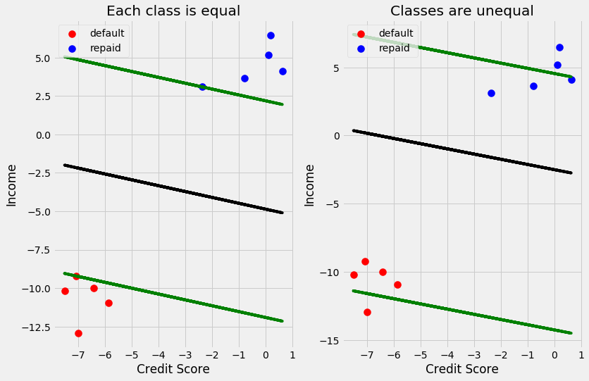
We can see the plot on the right, that the classifier is closer to the repaid. This will cause less values to be classified as repaid and limit the risk that the company is taking. This comes with the sacrifice of not giving some people loans that may repay their loans.