Feature Selection Using Boruta Algorithm
I am going to demonstrate how to use the Boruta algorithm for feature selection. To start I am going to show how to apply it to a dataset. I am going to make a dataset with 1000 samples and 4 features. Of those 4 features, only 2 of them will be useful. Lets see if Boruta is able to handle this.
Application
from sklearn.datasets import make_classification
import numpy as np
import pandas as pd

# make dataset
X, y = make_classification(n_samples = 1000,
                           n_features=4,
                           n_informative=2,
                           n_redundant=0,
                           random_state=11)

df = pd.DataFrame(X)
df['target'] = y
df.head()
| 0 | 1 | 2 | 3 | target | |
|---|---|---|---|---|---|
| 0 | -2.591025 | -1.223175 | 0.134147 | -1.788159 | 0 |
| 1 | 1.122498 | 1.180470 | -1.902731 | 0.065675 | 0 |
| 2 | 0.917016 | 0.935056 | -0.488524 | -0.598798 | 1 |
| 3 | 2.220961 | 0.015644 | 0.929275 | 0.548338 | 1 |
| 4 | 0.457067 | -1.481252 | -0.427098 | 2.119179 | 1 |
I am going to fit a RandomForest Classifier to this dataset.
from sklearn.ensemble import RandomForestClassifier

clf = RandomForestClassifier(max_depth=5)
Next import Boruta and run it
from boruta import BorutaPy

feat_selector = BorutaPy(clf, n_estimators='auto', verbose=1, random_state=1)
feat_selector.fit(X, y)
Iteration: 1 / 100
Iteration: 2 / 100
Iteration: 3 / 100
Iteration: 4 / 100
Iteration: 5 / 100
Iteration: 6 / 100
Iteration: 7 / 100
Iteration: 8 / 100
Iteration: 9 / 100
Iteration: 10 / 100
Iteration: 11 / 100
Iteration: 12 / 100
Iteration: 13 / 100
Iteration: 14 / 100
Iteration: 15 / 100
Iteration: 16 / 100
Iteration: 17 / 100
Iteration: 18 / 100
Iteration: 19 / 100
Iteration: 20 / 100
Iteration: 21 / 100
Iteration: 22 / 100
Iteration: 23 / 100
Iteration: 24 / 100
Iteration: 25 / 100
Iteration: 26 / 100
Iteration: 27 / 100
Iteration: 28 / 100
Iteration: 29 / 100
Iteration: 30 / 100
Iteration: 31 / 100
Iteration: 32 / 100
Iteration: 33 / 100
Iteration: 34 / 100
Iteration: 35 / 100
Iteration: 36 / 100
Iteration: 37 / 100
Iteration: 38 / 100
Iteration: 39 / 100
Iteration: 40 / 100
Iteration: 41 / 100
Iteration: 42 / 100
Iteration: 43 / 100
Iteration: 44 / 100
Iteration: 45 / 100
Iteration: 46 / 100
Iteration: 47 / 100
Iteration: 48 / 100
Iteration: 49 / 100


BorutaPy finished running.

Iteration: 	50 / 100
Confirmed: 	2
Tentative: 	0
Rejected: 	2


BorutaPy(alpha=0.05,
         estimator=RandomForestClassifier(bootstrap=True, class_weight=None,
                                          criterion='gini', max_depth=5,
                                          max_features='auto',
                                          max_leaf_nodes=None,
                                          min_impurity_decrease=0.0,
                                          min_impurity_split=None,
                                          min_samples_leaf=1,
                                          min_samples_split=2,
                                          min_weight_fraction_leaf=0.0,
                                          n_estimators=48, n_jobs=None,
                                          oob_score=False,
                                          random_state=<mtrand.RandomState object at 0x1a18f6f288>,
                                          verbose=0, warm_start=False),
         max_iter=100, n_estimators='auto', perc=100,
         random_state=<mtrand.RandomState object at 0x1a18f6f288>,
         two_step=True, verbose=1)
We see that it confirmed 2 of the features and rejected 2 features. Now lets see which features it is
feat_selector.support_
array([ True, True, False, False])
feat_selector.ranking_
array([1, 1, 3, 2])
Boruta says that the first and second feature are useful and I should remove the rest of the features. Now lets use the transform method to remove those features that are not useful.
X_filtered = feat_selector.transform(X)
X_filtered[:5]
array([[-2.5910246 , -1.22317524],
       [ 1.12249791,  1.18046999],
       [ 0.91701607,  0.93505646],
       [ 2.22096146,  0.01564356],
       [ 0.45706667, -1.48125216]])
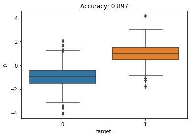
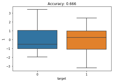
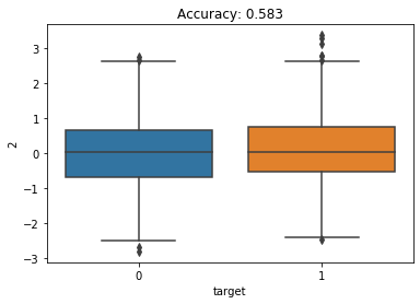
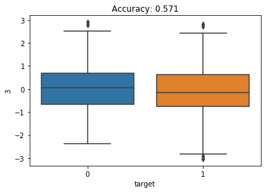
How can I tell check if Boruta did a good job or not. I am going to fit a random forest classifier on each individual feature with a small max depth (to prevent overfitting on the single feature). I’m also going to make boxplots showing the distribution of the feature for the 2 classes. I am expecting the first 2 features to have higher accuracy and have more separation between the 2 classes.
import seaborn as sns
import matplotlib.pyplot as plt
clf = RandomForestClassifier(max_depth=2)
for i in range(4):
    clf.fit(df[i].values.reshape(-1, 1), df['target'])
    sns.boxplot(x = 'target', y = i, data = df)
    plt.title(f"Accuracy: {clf.score(df[i].values.reshape(-1, 1), df['target'])}")
    plt.show()


We see that the first feature has a relatively high accuracy (90%) and the box plots show the 2 classes are very different for this feature. The second features has the next highest accuracy (67%). This makes sense why Boruta chose these as important features.
Theory
Now we will see the theory of Boruta.
Step 1: Make Permutations of each Feature
Boruta starts by taking permutations of each feature. I am going to call each of these new features a shadow.
np.random.seed(11)
X = df.drop('target', axis = 1)
X_shadow = X.apply(np.random.permutation)
X_shadow.columns = ['shadow_' + str(feat) for feat in X.columns]

X_boruta = pd.concat([X, X_shadow], axis = 1)
X_boruta.head()
| 0 | 1 | 2 | 3 | shadow_0 | shadow_1 | shadow_2 | shadow_3 | |
|---|---|---|---|---|---|---|---|---|
| 0 | -2.591025 | -1.223175 | 0.134147 | -1.788159 | -1.828319 | -0.636258 | 1.071065 | 0.385510 |
| 1 | 1.122498 | 1.180470 | -1.902731 | 0.065675 | 0.300768 | -2.208547 | 1.503905 | 0.355866 |
| 2 | 0.917016 | 0.935056 | -0.488524 | -0.598798 | -1.640707 | 0.505145 | -0.199718 | 1.827682 |
| 3 | 2.220961 | 0.015644 | 0.929275 | 0.548338 | -1.600522 | -0.667427 | 0.578215 | 0.629989 |
| 4 | 0.457067 | -1.481252 | -0.427098 | 2.119179 | -0.154074 | 0.631955 | 0.076234 | -1.896298 |
Step 2: Fit Random Forest Classifier to new dataset
I am now going to fit a random forest classifier to my new dataset and compare the feature importance of my original features to my datasets that have permutations
clf = RandomForestClassifier(max_depth = 5, random_state = 11)
clf.fit(X_boruta, y)
RandomForestClassifier(bootstrap=True, class_weight=None, criterion='gini',
                       max_depth=5, max_features='auto', max_leaf_nodes=None,
                       min_impurity_decrease=0.0, min_impurity_split=None,
                       min_samples_leaf=1, min_samples_split=2,
                       min_weight_fraction_leaf=0.0, n_estimators=10,
                       n_jobs=None, oob_score=False, random_state=11, verbose=0,
                       warm_start=False)
# feature importance of original features
feat_imp_X = clf.feature_importances_[:len(X.columns)]
feat_imp_X
array([0.66749262, 0.18664663, 0.03365685, 0.02609232])
# # feature importance of random data features
feat_imp_shadow = clf.feature_importances_[len(X.columns):]
feat_imp_shadow
array([0.02652004, 0.01652293, 0.02554006, 0.01752856])
Step 3: Compare feature importance of original dataset to random data
I now want to see which features have higher feature importance than most important random feature. The idea is that if a feature is not more important than the random features I should not include it. In the above example, the most important feature importance is 0.0265 - we see that this is greater than the last original feature because it has a feature importance of 0.0260. We can verify this with the below code:
hits = feat_imp_X > feat_imp_shadow.max()
hits
array([ True, True, True, False])
In this case, it says the first 3 features are useful and the last feature is not useful. However running this a single time, should not be trusted. We took random permutations of each feature so we should run this multiple times. When I used the Boruta package, it ran 50 iterations. I am now going to run it a second time with a different random seed.
np.random.seed(12)
X = df.drop('target', axis = 1)
X_shadow = X.apply(np.random.permutation)
X_shadow.columns = ['shadow_' + str(feat) for feat in X.columns]

X_boruta = pd.concat([X, X_shadow], axis = 1)
clf.fit(X_boruta, y)
feat_imp_X = clf.feature_importances_[:len(X.columns)]
feat_imp_shadow = clf.feature_importances_[len(X.columns):]
hits = feat_imp_X > feat_imp_shadow.max()
hits
array([ True, True, False, True])
We see that running it a second time, it gives a different subset of features to keep. I am now going to put this in a for loop and run it 20 times.
### repeat 20 times
hits = np.empty(4)
for iter_ in range(20):
   ### make X_shadow by randomly permuting each column of X
   np.random.seed(iter_)
   X_shadow = X.apply(np.random.permutation)
   X_boruta = pd.concat([X, X_shadow], axis = 1)
   ### fit a random forest (suggested max_depth between 3 and 7)
   clf = RandomForestClassifier(max_depth = 5, random_state = 42)
   clf.fit(X_boruta, y)
   ### store feature importance
   feat_imp_X = clf.feature_importances_[:len(X.columns)]
   feat_imp_shadow = clf.feature_importances_[len(X.columns):]
   ### compute hits for this trial and add to counter
   hits += (feat_imp_X > feat_imp_shadow.max()).astype(int)
hits / 20
array([1. , 1. , 0.1 , 0.15])
We see that of the 20 iterations feature 1 and feature 2 were selected every time. Feature 3 was selected 10% of the time and feature 4 was selected 15% of the time. The key component of Boruta is that instead of having the features compete against each other, they are competing against randomized versions of each other.