Interaction Terms Example

July 27, 2020

Below I am going to show the impact of making an interaction term.

I am going to begin my loading in the credit dataset

import pandas as pd

df = pd.read_csv('https://raw.githubusercontent.com/sik-flow/datasets/master/Credit.csv', index_col=0)
df.head()

	Income	Limit	Rating	Cards	Age	Education	Gender	Student	Married	Ethnicity	Balance
1	14.891	3606	283	2	34	11	Male	No	Yes	Caucasian	333
2	106.025	6645	483	3	82	15	Female	Yes	Yes	Asian	903
3	104.593	7075	514	4	71	11	Male	No	No	Asian	580
4	148.924	9504	681	3	36	11	Female	No	No	Asian	964
5	55.882	4897	357	2	68	16	Male	No	Yes	Caucasian	331

Make the Student column a dummy variable

df['Student'] = df['Student'].map(lambda x: 1 if x == 'Yes' else 0)

Use Income and Student to regress on Balance

import statsmodels.api as sm

X = df[['Income', 'Student']]
Y = df['Balance']

# coefficient 
X = sm.add_constant(X)

model = sm.OLS(Y, X).fit()
model.summary()

OLS Regression Results
Dep. Variable:	Balance	R-squared:	0.277
Model:	OLS	Adj. R-squared:	0.274
Method:	Least Squares	F-statistic:	76.22
Date:	Mon, 27 Jul 2020	Prob (F-statistic):	9.64e-29
Time:	20:06:40	Log-Likelihood:	-2954.4
No. Observations:	400	AIC:	5915.
Df Residuals:	397	BIC:	5927.
Df Model:	2
Covariance Type:	nonrobust

	coef	std err	t	P>\|t\|	[0.025	0.975]
const	211.1430	32.457	6.505	0.000	147.333	274.952
Income	5.9843	0.557	10.751	0.000	4.890	7.079
Student	382.6705	65.311	5.859	0.000	254.272	511.069

Omnibus:	119.719	Durbin-Watson:	1.951
Prob(Omnibus):	0.000	Jarque-Bera (JB):	23.617
Skew:	0.252	Prob(JB):	7.44e-06
Kurtosis:	1.922	Cond. No.	192.

Warnings:
[1] Standard Errors assume that the covariance matrix of the errors is correctly specified.

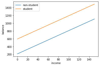
Now I am going to plot out the regression lines for when someone is a student and when someone is not a student

import numpy as np
import matplotlib.pyplot as plt

Xnew = np.array([[1, 0, 0], [1, 150, 0], [1, 0, 1], [1, 150, 1]])
preds = model.predict(Xnew)

plt.plot([0, 150], preds[:2], label = 'non-student')
plt.plot([0, 150], preds[2:], label = 'student')
plt.xlabel('income')
plt.ylabel('balance')
plt.legend()

<matplotlib.legend.Legend at 0x1c1dbafb70>

png

I see that the 2 lines are parallel. The balance for students and non students both increase at the same rate as income increases. But what if that is not the case? That is where an interaction term comes into use.

I am going to make an interaction term between student and income.

df['Interaction'] = df['Student'] * df['Income']

X = df[['Income', 'Student', 'Interaction']]
Y = df['Balance']

# coefficient 
X = sm.add_constant(X)

model = sm.OLS(Y, X).fit()
model.summary()

OLS Regression Results
Dep. Variable:	Balance	R-squared:	0.280
Model:	OLS	Adj. R-squared:	0.274
Method:	Least Squares	F-statistic:	51.30
Date:	Mon, 27 Jul 2020	Prob (F-statistic):	4.94e-28
Time:	20:07:38	Log-Likelihood:	-2953.7
No. Observations:	400	AIC:	5915.
Df Residuals:	396	BIC:	5931.
Df Model:	3
Covariance Type:	nonrobust

	coef	std err	t	P>\|t\|	[0.025	0.975]
const	200.6232	33.698	5.953	0.000	134.373	266.873
Income	6.2182	0.592	10.502	0.000	5.054	7.382
Student	476.6758	104.351	4.568	0.000	271.524	681.827
Interaction	-1.9992	1.731	-1.155	0.249	-5.403	1.404

Omnibus:	107.788	Durbin-Watson:	1.952
Prob(Omnibus):	0.000	Jarque-Bera (JB):	22.158
Skew:	0.228	Prob(JB):	1.54e-05
Kurtosis:	1.941	Cond. No.	309.

Warnings:
[1] Standard Errors assume that the covariance matrix of the errors is correctly specified.

Xnew = np.array([[1, 0, 0, 0], [1, 150, 0, 0], [1, 0, 1, 0], [1, 150, 1, 150]])
preds = model.predict(Xnew)

plt.plot([0, 150], preds[:2], label = 'non-student')
plt.plot([0, 150], preds[2:], label = 'student')
plt.xlabel('income')
plt.ylabel('balance')
plt.legend()

<matplotlib.legend.Legend at 0x1c1dc9e4a8>

png

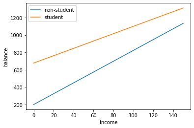
Now we see that the the 2 lines have different slopes. The slope for students is lower than the slope for non-students. This suggestions that increases in income are associated with smaller increases in credit card balance among students as compared to non-students.