Checking for Linearity with Residual Plots

July 26, 2020

We can use residual plots to determine if there is a non-linear relationship. I am going to demonstrate this using the Auto dataset.

First load in the dataset

import pandas as pd
import seaborn as sns 
import matplotlib.pyplot as plt
import numpy as np

df = pd.read_csv('https://raw.githubusercontent.com/sik-flow/datasets/master/auto-mpg.csv')

# remove missing values in horsepower
df = df[df['horsepower'] != '?']
df['horsepower'] = df['horsepower'].astype(float)

import statsmodels.formula.api as smf

Now I am going to fit a model with all of the below features

model = 'mpg ~ cylinders + \
                 displacement + \
                 horsepower + \
                 weight + \
                 acceleration + \
                 origin'

model = smf.ols(formula=model, data=df)
model_fit = model.fit()
model_fitted_y = model_fit.fittedvalues

sns.residplot(model_fitted_y, 'mpg', data=df, 
                          lowess=True, 
                          scatter_kws={'alpha': 0.5}, 
                          line_kws={'color': 'red', 'lw': 1, 'alpha': 0.8})
plt.xlabel('Fitted Values')
plt.ylabel('Residuals');

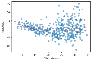
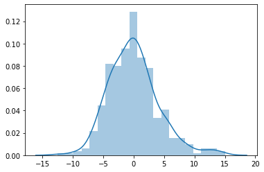
The red line is fitted to the points. I am looking for this line to be roughly straight along the 0 line of the residuals. We see that this line is close to be straight. We can verify the residuals using a density plot.

sns.distplot(model_fit.resid)

<matplotlib.axes._subplots.AxesSubplot at 0x1a2dcc8550>

Residuals appear to be normal.

Lets see what it looks like when we have a non-linear relationship between the independent and dependent variable.

model = 'mpg ~ horsepower'

model = smf.ols(formula=model, data=df)
model_fit = model.fit()
model_fitted_y = model_fit.fittedvalues

sns.residplot(model_fitted_y, 'mpg', data=df, 
                          lowess=True, 
                          scatter_kws={'alpha': 0.5}, 
                          line_kws={'color': 'red', 'lw': 1, 'alpha': 0.8})
plt.xlabel('Fitted Values')
plt.ylabel('Residuals');

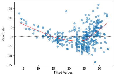
Now we see the red line makes a U pattern - this indicates there is a non-linear relationship between the independent variable and dependent variable. To combat this I would recommend trying to transform the independent with log(X), sqrt(X), or X^2.