Simple GAM with PyGAM
Show how to implement a GAM using PyGam
Start with loading in a dataset
from pygam.datasets import wage

X, y = wage()
Fit a GAM - first 2 features will be using a spline term and the 3rd feature will be using a factor term.
from pygam import LinearGAM, s, f

gam = LinearGAM(s(0) + s(1) + f(2)).fit(X, y)
gam.summary()
LinearGAM
=============================================== ==========================================================
Distribution:                        NormalDist Effective DoF:                                     25.1911
Link Function:                     IdentityLink Log Likelihood:                                -24118.6847
Number of Samples:                         3000 AIC:                                            48289.7516
                                                AICc:                                           48290.2307
                                                GCV:                                             1255.6902
                                                Scale:                                           1236.7251
                                                Pseudo R-Squared:                                   0.2955
==========================================================================================================
Feature Function                  Lambda               Rank         EDoF         P > x        Sig. Code
================================= ==================== ============ ============ ============ ============
s(0)                              [0.6]                20           7.1          5.95e-03     **
s(1)                              [0.6]                20           14.1         1.11e-16     ***
f(2)                              [0.6]                5            4.0          1.11e-16     ***
intercept                                              1            0.0          1.11e-16     ***
==========================================================================================================
Significance codes:  0 '***' 0.001 '**' 0.01 '*' 0.05 '.' 0.1 ' ' 1

WARNING: Fitting splines and a linear function to a feature introduces a model identifiability problem
         which can cause p-values to appear significant when they are not.

WARNING: p-values calculated in this manner behave correctly for un-penalized models or models with
         known smoothing parameters, but when smoothing parameters have been estimated, the p-values
         are typically lower than they should be, meaning that the tests reject the null too readily.


/Users/jeffreyherman/opt/anaconda3/lib/python3.7/site-packages/ipykernel_launcher.py:1: UserWarning: KNOWN BUG: p-values computed in this summary are likely much smaller than they should be.

Please do not make inferences based on these values!

Collaborate on a solution, and stay up to date at:
github.com/dswah/pyGAM/issues/163

  """Entry point for launching an IPython kernel.
gam.lam
[[0.6], [0.6], [0.6]]
We see the lambda term for each feature is 0.6. I am going to tune this using gridsearch.
import numpy as np

lam = np.logspace(-3, 5, 5)
lams = [lam] * 3

gam.gridsearch(X, y, lam=lams)
gam.summary()
100% (125 of 125) |######################| Elapsed Time: 0:00:03 Time:  0:00:03


LinearGAM
=============================================== ==========================================================
Distribution:                        NormalDist Effective DoF:                                      9.6668
Link Function:                     IdentityLink Log Likelihood:                                 -24119.413
Number of Samples:                         3000 AIC:                                            48260.1595
                                                AICc:                                           48260.2428
                                                GCV:                                             1244.2375
                                                Scale:                                           1237.0229
                                                Pseudo R-Squared:                                   0.2916
==========================================================================================================
Feature Function                  Lambda               Rank         EDoF         P > x        Sig. Code
================================= ==================== ============ ============ ============ ============
s(0)                              [100000.]            20           2.4          9.04e-03     **
s(1)                              [1000.]              20           3.3          1.11e-16     ***
f(2)                              [0.1]                5            3.9          1.11e-16     ***
intercept                                              1            0.0          1.11e-16     ***
==========================================================================================================
Significance codes:  0 '***' 0.001 '**' 0.01 '*' 0.05 '.' 0.1 ' ' 1

WARNING: Fitting splines and a linear function to a feature introduces a model identifiability problem
         which can cause p-values to appear significant when they are not.

WARNING: p-values calculated in this manner behave correctly for un-penalized models or models with
         known smoothing parameters, but when smoothing parameters have been estimated, the p-values
         are typically lower than they should be, meaning that the tests reject the null too readily.


/Users/jeffreyherman/opt/anaconda3/lib/python3.7/site-packages/ipykernel_launcher.py:7: UserWarning: KNOWN BUG: p-values computed in this summary are likely much smaller than they should be.

Please do not make inferences based on these values!

Collaborate on a solution, and stay up to date at:
github.com/dswah/pyGAM/issues/163

  import sys
Now lets see the partial dependence plots of our features
import matplotlib.pyplot as plt

for i, term in enumerate(gam.terms):
    if term.isintercept:
        continue

    XX = gam.generate_X_grid(term=i)
    pdep, confi = gam.partial_dependence(term=i, X=XX, width=0.95)

    plt.figure()
    plt.plot(XX[:, term.feature], pdep)
    plt.plot(XX[:, term.feature], confi, c='r', ls='--')
    plt.title(repr(term))
    plt.show()


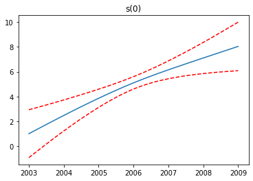
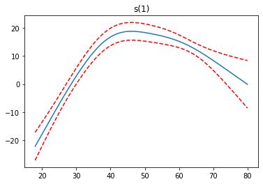
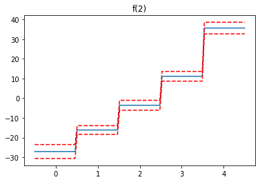
We see the first feature has a steady increase, the second feature increases to a point, then levels off and finally decreases, while the third feature increases.
Now I am going to compare the performance vs linear regression
from sklearn.model_selection import train_test_split
X_train, X_test, y_train, y_test = train_test_split(X, y, test_size=0.25, random_state=11)
gam = LinearGAM(s(0) + s(1) + f(2)).fit(X, y)

lam = np.logspace(-3, 5, 5)
lams = [lam] * 3

gam.gridsearch(X_train, y_train, lam=lams)
gam.summary()
100% (125 of 125) |######################| Elapsed Time: 0:00:03 Time:  0:00:03


LinearGAM
=============================================== ==========================================================
Distribution:                        NormalDist Effective DoF:                                      9.3578
Link Function:                     IdentityLink Log Likelihood:                                -18073.3788
Number of Samples:                         2250 AIC:                                            36167.4732
                                                AICc:                                           36167.5783
                                                GCV:                                             1237.4156
                                                Scale:                                           1228.1554
                                                Pseudo R-Squared:                                   0.2918
==========================================================================================================
Feature Function                  Lambda               Rank         EDoF         P > x        Sig. Code
================================= ==================== ============ ============ ============ ============
s(0)                              [100000.]            20           2.3          5.58e-02     .
s(1)                              [1000.]              20           3.1          1.11e-16     ***
f(2)                              [0.1]                5            3.9          1.11e-16     ***
intercept                                              1            0.0          1.11e-16     ***
==========================================================================================================
Significance codes:  0 '***' 0.001 '**' 0.01 '*' 0.05 '.' 0.1 ' ' 1

WARNING: Fitting splines and a linear function to a feature introduces a model identifiability problem
         which can cause p-values to appear significant when they are not.

WARNING: p-values calculated in this manner behave correctly for un-penalized models or models with
         known smoothing parameters, but when smoothing parameters have been estimated, the p-values
         are typically lower than they should be, meaning that the tests reject the null too readily.


/Users/jeffreyherman/opt/anaconda3/lib/python3.7/site-packages/ipykernel_launcher.py:7: UserWarning: KNOWN BUG: p-values computed in this summary are likely much smaller than they should be.

Please do not make inferences based on these values!

Collaborate on a solution, and stay up to date at:
github.com/dswah/pyGAM/issues/163

  import sys
from sklearn.metrics import mean_squared_error

mean_squared_error(y_test, gam.predict(X_test))
1265.8585409629538
import pandas as pd

df_train = pd.DataFrame(X_train)
df_train['Y'] = y_train
df_train.columns = ['X1', 'X2', 'X3', 'Y']

df_test = pd.DataFrame(X_test)
df_test['Y'] = y_test
df_test.columns = ['X1', 'X2', 'X3', 'Y']
df_train.head()
| X1 | X2 | X3 | Y | |
|---|---|---|---|---|
| 0 | 2009.0 | 56.0 | 0.0 | 79.854900 |
| 1 | 2005.0 | 45.0 | 2.0 | 81.283253 |
| 2 | 2008.0 | 33.0 | 1.0 | 128.680488 |
| 3 | 2006.0 | 51.0 | 4.0 | 153.457515 |
| 4 | 2005.0 | 29.0 | 3.0 | 128.680488 |
from statsmodels.formula.api import ols
formula = 'Y ~ X1 + X2 + C(X3)'
model = ols(formula=formula, data=df_train).fit()
model.summary()
| Dep. Variable: | Y | R-squared: | 0.258 |
|---|---|---|---|
| Model: | OLS | Adj. R-squared: | 0.256 |
| Method: | Least Squares | F-statistic: | 130.3 |
| Date: | Sat, 08 Aug 2020 | Prob (F-statistic): | 9.99e-142 |
| Time: | 21:04:36 | Log-Likelihood: | -11242. |
| No. Observations: | 2250 | AIC: | 2.250e+04 |
| Df Residuals: | 2243 | BIC: | 2.254e+04 |
| Df Model: | 6 | ||
| Covariance Type: | nonrobust |
| coef | std err | t | P>|t| | [0.025 | 0.975] | |
|---|---|---|---|---|---|---|
| Intercept | -1906.3133 | 745.462 | -2.557 | 0.011 | -3368.182 | -444.445 |
| C(X3)[T.1.0] | 10.0980 | 2.929 | 3.447 | 0.001 | 4.353 | 15.842 |
| C(X3)[T.2.0] | 21.2259 | 3.060 | 6.936 | 0.000 | 15.224 | 27.228 |
| C(X3)[T.3.0] | 38.9505 | 3.055 | 12.749 | 0.000 | 32.959 | 44.942 |
| C(X3)[T.4.0] | 62.7525 | 3.282 | 19.118 | 0.000 | 56.316 | 69.189 |
| X1 | 0.9817 | 0.372 | 2.641 | 0.008 | 0.253 | 1.711 |
| X2 | 0.5522 | 0.066 | 8.371 | 0.000 | 0.423 | 0.682 |
| Omnibus: | 667.758 | Durbin-Watson: | 2.000 |
|---|---|---|---|
| Prob(Omnibus): | 0.000 | Jarque-Bera (JB): | 3095.965 |
| Skew: | 1.347 | Prob(JB): | 0.00 |
| Kurtosis: | 8.076 | Cond. No. | 1.98e+06 |
Warnings:
[1] Standard Errors assume that the covariance matrix of the errors is correctly specified.
[2] The condition number is large, 1.98e+06. This might indicate that there are
strong multicollinearity or other numerical problems.
mean_squared_error(df_test['Y'], model.predict(dict(X1 = df_test['X1'].values,
                                                    X2 = df_test['X2'].values,
                                                   X3 = df_test['X3'].values)))
1300.8156546398066
We see the GAM has a lower MSE