Clustering - Spectral Clustering
Spectral clustering is a technique with roots in graph theory, where the approach is used to identify communities of nodes in a graph based on the edges connecting them. The method is flexible and allows us to cluster non-graph data as well. [source]
Motivating Example
Let’s start with a motivating example. We have the following data:
from sklearn import cluster, datasets
import matplotlib.pyplot as plt

noisy_circles = datasets.make_circles(n_samples=1000, factor=.5,
                                      noise=.05, random_state = 11)

plt.scatter(noisy_circles[0][:, 0], noisy_circles[0][:, 1]);
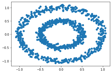
We can see there are 2 clusters, the inner circle, and the outer circle. Now, let’s see how k-means does in clustering the data.
from sklearn.cluster import KMeans

kmeans = KMeans(n_clusters = 2)

clusters = kmeans.fit(noisy_circles[0]).predict(noisy_circles[0])

plt.scatter(noisy_circles[0][:, 0], noisy_circles[0][:, 1], c = clusters);
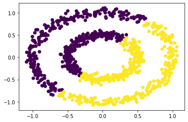
After performing K-Means we see it does not cluster the data based on the circles but instead, clusters based on the overall location of the different data points.
Now using the same dataset, let’s try spectral clustering.
from sklearn.cluster import SpectralClustering

spectral = cluster.SpectralClustering(
        n_clusters=2, affinity = 'nearest_neighbors')

spec_clusters = spectral.fit(noisy_circles[0]).labels_

plt.scatter(noisy_circles[0][:, 0], noisy_circles[0][:, 1], c = spec_clusters);

We see that spectral clustering is able to capture the groups of circles.
How Does it Work?
Remember from the introduction, spectral clustering has its roots in graph theory - so I am going to start out with the following example.
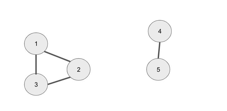
We have 5 nodes, the first 3 are all connected to each other and the last 2 are connected to each other. To perform spectral clustering on these data points we need to perform the following steps:
- Make adjacency matrix from the graph
- Make Laplacian matrix from the graph
- Calculate Eigenvectors of Laplacian matrix
- Perform K-Means clustering on the k-smallest Eigenvectors
Step 1: Make adjacency matrix from the graph
import numpy as np

adjacency_matrix = np.matrix([[0, 1, 1, 0, 0],
                              [1, 0, 1, 0, 0],
                              [1, 1, 0, 0, 0],
                              [0, 0, 0, 0, 1],
                              [0, 0, 0, 1, 0]])
adjacency_matrix
matrix([[0, 1, 1, 0, 0],
        [1, 0, 1, 0, 0],
        [1, 1, 0, 0, 0],
        [0, 0, 0, 0, 1],
        [0, 0, 0, 1, 0]])
An adjacency is used to represent a graph. For example, the first row [0, 1, 1, 0, 0], means that node 1 is connected to nodes 2 and 3 and is not connected to nodes 1, 4, and 5.
Step 2: Make Laplacian matrix from the graph
The Laplacian matrix can be calculated by the following formula
\[L = D - A\]Where D is the degree matrix and A is the adjacency matrix
# make degree matrix
degree_matrix = np.zeros((5, 5))
np.fill_diagonal(degree_matrix, np.sum(adjacency_matrix, axis=1))

degree_matrix
array([[2., 0., 0., 0., 0.],
       [0., 2., 0., 0., 0.],
       [0., 0., 2., 0., 0.],
       [0., 0., 0., 1., 0.],
       [0., 0., 0., 0., 1.]])
# make Laplacian matrix

laplacian = degree_matrix - adjacency_matrix
laplacian
matrix([[ 2., -1., -1.,  0.,  0.],
        [-1.,  2., -1.,  0.,  0.],
        [-1., -1.,  2.,  0.,  0.],
        [ 0.,  0.,  0.,  1., -1.],
        [ 0.,  0.,  0., -1.,  1.]])
As a sanity check, we can verify the Laplacian Matrix is calculated correctly by using NetworkX
import networkx as nx

G = nx.from_numpy_matrix(adjacency_matrix)
nx.laplacian_matrix(G).toarray()
array([[ 2, -1, -1,  0,  0],
       [-1,  2, -1,  0,  0],
       [-1, -1,  2,  0,  0],
       [ 0,  0,  0,  1, -1],
       [ 0,  0,  0, -1,  1]])
Step 3: Calculate Eigenvectors of Laplacian matrix
eig_vals, eig_vectors = np.linalg.eig(laplacian)

# eigenvalues
print('Eigenvalues')
print(eig_vals.round(2))
print('--'*15)
print('Eigenvectors')
print(eig_vectors)
Eigenvalues
[ 3. -0.  3.  2.  0.]
------------------------------
Eigenvectors
[[ 0.81649658 -0.57735027  0.29329423  0.          0.        ]
 [-0.40824829 -0.57735027 -0.80655913  0.          0.        ]
 [-0.40824829 -0.57735027  0.5132649   0.          0.        ]
 [ 0.          0.          0.          0.70710678  0.70710678]
 [ 0.          0.          0.         -0.70710678  0.70710678]]
A couple of points to notice - when looking at the Eigenvectors we see the first 3 vectors are similar and the last 2 vectors are similar. This will be useful during Step 5 when we use K-Means on the Eigenvectors to form the clusters. Another point of notice, we 2 Eigenvalues that are 0. In a Laplacian matrix the number of 0 Eigenvalues corresponds to the number of connected components in our graph. Take a look at the below gif.
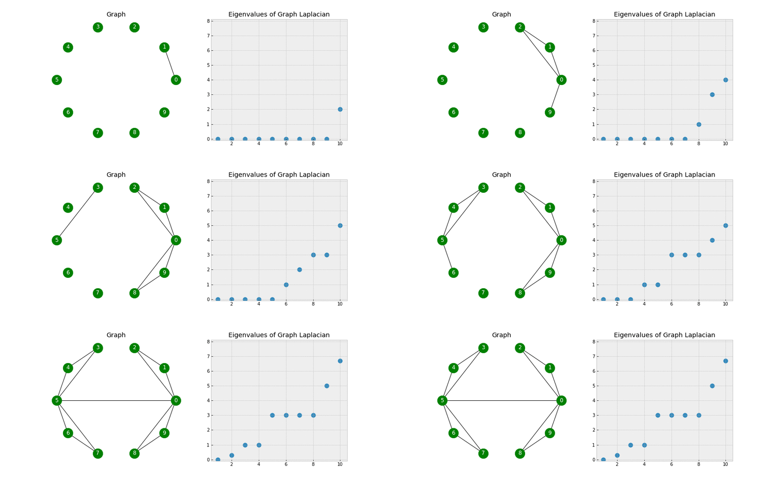
As we start connecting points, we see the number of non-zero Eigenvalues increase. This is because the number of clusters is decreasing (when no points are connected we have 10 clusters, when there is one connection we have 9 clusters, etc).
Step 4: Perform K-Means clustering on the k-smallest Eigenvectors
I will be using k = 2
eig_vals
array([ 3.0000000e+00, -4.4408921e-16,  3.0000000e+00,  2.0000000e+00,
        0.0000000e+00])
eig_vectors
matrix([[ 0.81649658, -0.57735027,  0.29329423,  0.        ,  0.        ],
        [-0.40824829, -0.57735027, -0.80655913,  0.        ,  0.        ],
        [-0.40824829, -0.57735027,  0.5132649 ,  0.        ,  0.        ],
        [ 0.        ,  0.        ,  0.        ,  0.70710678,  0.70710678],
        [ 0.        ,  0.        ,  0.        , -0.70710678,  0.70710678]])
eig_vectors[:, np.argsort(eig_vals)[:k]]
matrix([[-0.57735027,  0.        ],
        [-0.57735027,  0.        ],
        [-0.57735027,  0.        ],
        [ 0.        ,  0.70710678],
        [ 0.        ,  0.70710678]])
k = 2

k_eig_vectors = eig_vectors[:, np.argsort(eig_vals)[:k]]

kmeans = KMeans(n_clusters = 2)

kmeans.fit(k_eig_vectors).predict(k_eig_vectors)
array([1, 1, 1, 0, 0], dtype=int32)
We see the first 3 data points are part of a cluster and the last 2 data points are part of another cluster, this matches up with our original data.
Now let’s return to our original dataset (the circles), how would we apply these steps to that dataset since our data is not in a graph? We could consider points to be “connected” based on their distance and the nearest points would be connected.
from sklearn.neighbors import kneighbors_graph

# step 1 - create adjacency matrix
adjacency_matrix = kneighbors_graph(noisy_circles[0], n_neighbors=7).toarray()

# step 2 - create Laplacian matrix
degree_matrix = np.diag(adjacency_matrix.sum(axis=1))
laplacian_matrix = degree_matrix - adjacency_matrix

# step 3 - calculate eigenvectors and values
eig_vals, eig_vecs = np.linalg.eig(laplacian_matrix)
eig_vals = eig_vals.real
eig_vecs = eig_vecs.real

# step 4 - perform k-means clustering on the k-smallest eigenvectors
k_eig_vectors = vecs[:, np.argsort(vals)[:k]]
kmeans = KMeans(n_clusters = 2)
clusters = kmeans.fit(k_eig_vectors).predict(k_eig_vectors)

plt.scatter(noisy_circles[0][:, 0], noisy_circles[0][:, 1], c = preds);
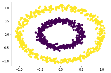
We get the same results as using the sklearn package.