Example and Visualization of Tukey Test
A Tukey Test is a way to compare more than 2 datasets and see which are statistically significant. I will demo this using the Auto MPG Dataset from UCI
import pandas as pd

# load in dataset
df = pd.read_csv('auto-mpg.csv')

# update orgin column
df.loc[df['origin'] == 1, 'origin'] = 'US'
df.loc[df['origin'] == 2, 'origin'] = 'Germany'
df.loc[df['origin'] == 3, 'origin'] = 'Japan'

df.head()
| mpg | cylinders | displacement | horsepower | weight | acceleration | model year | origin | car name | |
|---|---|---|---|---|---|---|---|---|---|
| 0 | 18.0 | 8 | 307.0 | 130 | 3504 | 12.0 | 70 | US | chevrolet chevelle malibu |
| 1 | 15.0 | 8 | 350.0 | 165 | 3693 | 11.5 | 70 | US | buick skylark 320 |
| 2 | 18.0 | 8 | 318.0 | 150 | 3436 | 11.0 | 70 | US | plymouth satellite |
| 3 | 16.0 | 8 | 304.0 | 150 | 3433 | 12.0 | 70 | US | amc rebel sst |
| 4 | 17.0 | 8 | 302.0 | 140 | 3449 | 10.5 | 70 | US | ford torino |
I want to see if the number of cylinders is statistically different depending on the origin of the car.
from statsmodels.stats.multicomp import MultiComparison

cardata = MultiComparison(df['cylinders'], df['origin'])
results = cardata.tukeyhsd()
results.summary()
| group1 | group2 | meandiff | p-adj | lower | upper | reject |
|---|---|---|---|---|---|---|
| Germany | Japan | -0.0559 | 0.9 | -0.5805 | 0.4688 | False |
| Germany | US | 2.0919 | 0.001 | 1.6595 | 2.5242 | True |
| Japan | US | 2.1477 | 0.001 | 1.735 | 2.5605 | True |
We see that the number of cylinders in cars that originated in Germany and Japan are not statistically significant, we also see that cars that originated in the US have a statistcally different number of cylinders than cars that originated in Japan or Germany.
Now lets visualize this.
results.plot_simultaneous();
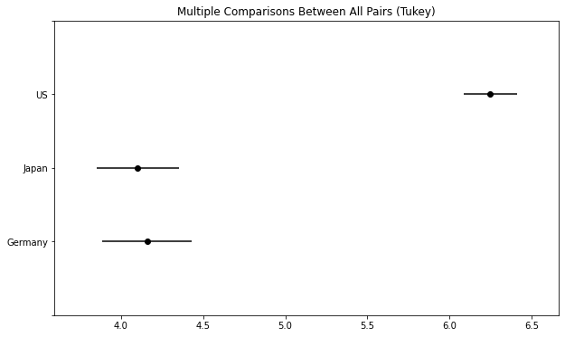
The X-Axis is the number of cylinders and we see why the US had a statistically significant result, due to having a much higher mean number of cylinders.
We can also highlight one of the groups using comparison_name. I’m going to highlight Japan.
results.plot_simultaneous(comparison_name = 'Japan');
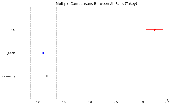
This shows that Germany intersects the confidence interval of Germany and this is why they were not statistically different.