Testing Multicollinearity with VIF
Multicollinearity is where 3 or more features are highly correlated. I am going to demonstrate how to calculate when you are experiencing multicollinearity using variance inflation factor (VIF).
To start I am going to use sklearn to make a dataset.
from sklearn.datasets import make_regression
import pandas as pd
import numpy as np
np.random.seed(11)
X, y = make_regression(n_features = 10, noise=10, random_state=11, )
df = pd.DataFrame(X, columns=['X1', 'X2', 'X3', 'X4', 'X5', 'X6', 'X7', 'X8', 'X9', 'X10'])
df['Y'] = y
I am going to create a new feature that is a combination of the other features.
df['X11'] = df['X1'] - df['X2'] + df['X3'] + np.random.normal(scale = 15)
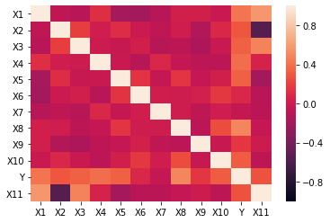
Now lets look at the correlation heat map to see if there is any highly correlated features.
import seaborn as sns
sns.heatmap(df.corr(), vmin = -1, vmax = 1)
<matplotlib.axes._subplots.AxesSubplot at 0x1c2ebcc590>

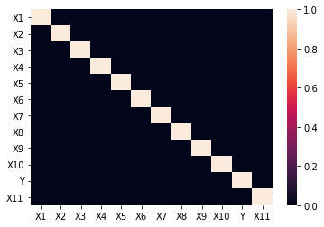
sns.heatmap(np.abs(df.corr()) > 0.7)
<matplotlib.axes._subplots.AxesSubplot at 0x1c2e9c38d0>

We see that none of the features have a correlation above 0.70 or below -0.70. Next, I am going to use VIF to determine if I am experiencing multicollinearity.
from statsmodels.stats.outliers_influence import variance_inflation_factor
Note: per this open issue on variance inflation factor you need to add a constant variable to your dataframe.
df = sm.add_constant(df)
I am going to test out all the features to see what the VIF value is. I am skipping the first feature (the intercept term).
for i in range(1, 12):
    print(f'{df.drop("Y", axis = 1).columns[i]} {variance_inflation_factor(df.drop("Y", axis = 1).values, i)}')
X1 inf
X2 inf
X3 inf
X4 1.0410536144535685
X5 1.0917593842615227
X6 1.0955635908289258
X7 1.0425296201253647
X8 1.1118123228822059
X9 1.051488347630868
X10 1.1173223003485167
X11 inf
I see I have multiple features that have a VIF value of inf. Lets see what is causing that.
Below is the formula for how VIF is calculated.
\[VIF = \frac{1}{1 - R^2}\]From above, I got a VIF of inf for X1. To calculate VIF for X1 - I am going to build a regression using all the independent variables except for X1 and use those features to predict X1.
X = df.drop(['X1', 'Y'], axis = 1)
Y = df['X1']

model = sm.OLS(Y, X).fit()
model.summary()
| Dep. Variable: | X1 | R-squared: | 1.000 |
|---|---|---|---|
| Model: | OLS | Adj. R-squared: | 1.000 |
| Method: | Least Squares | F-statistic: | 1.305e+27 |
| Date: | Sun, 26 Jul 2020 | Prob (F-statistic): | 0.00 |
| Time: | 16:55:53 | Log-Likelihood: | 2874.8 |
| No. Observations: | 100 | AIC: | -5728. |
| Df Residuals: | 89 | BIC: | -5699. |
| Df Model: | 10 | ||
| Covariance Type: | nonrobust |
| coef | std err | t | P>|t| | [0.025 | 0.975] | |
|---|---|---|---|---|---|---|
| const | -26.2418 | 2.42e-13 | -1.08e+14 | 0.000 | -26.242 | -26.242 |
| X2 | 1.0000 | 1.26e-14 | 7.92e+13 | 0.000 | 1.000 | 1.000 |
| X3 | -1.0000 | 1.18e-14 | -8.47e+13 | 0.000 | -1.000 | -1.000 |
| X4 | -3.816e-16 | 8.28e-15 | -0.046 | 0.963 | -1.68e-14 | 1.61e-14 |
| X5 | 3.088e-16 | 9.08e-15 | 0.034 | 0.973 | -1.77e-14 | 1.84e-14 |
| X6 | 2.984e-16 | 9.72e-15 | 0.031 | 0.976 | -1.9e-14 | 1.96e-14 |
| X7 | -1.388e-17 | 8.44e-15 | -0.002 | 0.999 | -1.68e-14 | 1.68e-14 |
| X8 | 1.596e-16 | 8.42e-15 | 0.019 | 0.985 | -1.66e-14 | 1.69e-14 |
| X9 | -6.635e-17 | 8.85e-15 | -0.007 | 0.994 | -1.77e-14 | 1.75e-14 |
| X10 | -2.533e-16 | 8.44e-15 | -0.030 | 0.976 | -1.7e-14 | 1.65e-14 |
| X11 | 1.0000 | 9.2e-15 | 1.09e+14 | 0.000 | 1.000 | 1.000 |
| Omnibus: | 0.540 | Durbin-Watson: | 0.009 |
|---|---|---|---|
| Prob(Omnibus): | 0.763 | Jarque-Bera (JB): | 0.660 |
| Skew: | 0.157 | Prob(JB): | 0.719 |
| Kurtosis: | 2.757 | Cond. No. | 761. |
Warnings:
[1] Standard Errors assume that the covariance matrix of the errors is correctly specified.
I see that I get a perfect R^2. So plugging this into my VIF formula
\[VIF = \frac{1}{1 - 1}\]This is where the inf comes from. I have a problem because I am able to perfectly predict X1 from the other features. Now lets see what happens when I remove the feature I created.
df.drop(['Y', 'X11'], axis = 1, inplace = True)
for i in range(1, 11):
    print(f'{df.columns[i]} {variance_inflation_factor(df.values, i)}')
X1 1.1056812354246772
X2 1.0741738574018993
X3 1.0836168289787529
X4 1.0410536144535685
X5 1.0917593842615227
X6 1.0955635908289256
X7 1.0425296201253647
X8 1.1118123228822059
X9 1.051488347630868
X10 1.1173223003485164
Now, I see that I get value for each of the 10 features. We typically use a threshold of either below 5 or below 10 as a good VIF. A VIF of 5 means that the other features are able to predict that feature with a R^2 of 0.80. A VIF of 10 means that the other features are able to predict that feature with a R^2 of 0.90.